Tutorial 1 - Using the demo database to get to know the STEMgis Viewer
When you first install STEMgis, STEMgis Viewer will open up the demo database provided with the software. Thereafter, the Viewer will open the last database that was used within the Viewer. If you need to relocate the demo database you will find it in a sub-directory wherever you installed STEMgis. For example if you installed STEMgis in c:\Program Files\Discovery Software\STEMgis then you will find the demo database at c:\Program Files\Discovery Software\STEMgis\data\dbase\demoSg.mdb. Use File->Open Database to open a STEMgis database.
STEMgis Layout
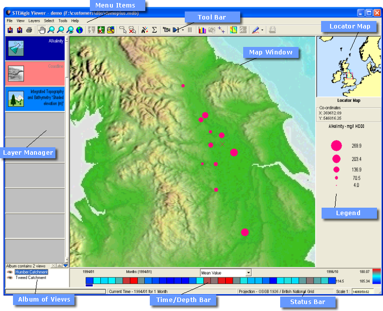
The figure below highlights the layout of STEMgis:

While the following image shows the functionality of the toolbar for STEMgis:

Accessing data
One of the main advantages of STEMgis over other mapping software is the ability to handle data that are dynamic over time. STEMgis achieves this by attaching time information to all locational and attribute data and by storing all of these data within one database.
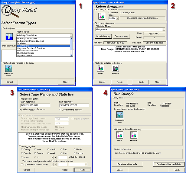
STEMgis provides a simple (at most four stage) process to accessing data from this database, via the Query Wizard (see toolbar above).
The graphic shows the stages involved, i.e. selecting feature types, selecting attributes, selecting time ranges and retrieving the data:

Visualizing the Data
Once you have retrieved data from the database you can visualize it many different ways, e.g.:
Traffic Volume Data
|
Step 1: To retrieve Landmark/OS Raster Maps. Click on the Query Wizard icon, select Landmark & Ordnance Survey 1:10560 raster maps from the list, click on Include in Query and click on Next. Select OS 1:10560 raster maps as the attribute, click on Include in Query and click on Next. On the following screen click on Next and then subsequently click on Retrieve sites and data. On the Query Results screen click on Finish. A new layer will have appeared in the Layer Manager. Don't worry that you can't see anything on the map just yet. Step 2: Using a similar procedure as above, retrieve Traffic Data, select Traffic Volume as the attribute and aggregate to an hourly period (click on the hour radio button on the Select Time Range and Statistics screen). Tip: Select Traffic Volume as the current layer (left click on the layer in the layer manager) and then Zoom to current layer via the View Menu. Tip: Dark blue shading in the layer manager indicates which layer is currently selected. Step 3: Select the raster maps as current layer. Tip: To give a white background to the raster maps turn off the image transparency (View Menu -> Options) Step 4: Use the time bar to select 1950 map (each period of time is represented by a different colour - in this case 1950 is green). Note: You are looking at purely simulated data designed to reflect the functionality of STEMgis rather than bear any resemblance of reality on New Year's day, 1950! Step 5: Select Traffic Volume as current layer and animate using animate icon. Click on the play button to start the animation and on the pause button to stop. Step 6: Graph data for one road by selecting the graphing icon from the toolbar and then clicking on a road. |
Water Quality Data
|
Step 1: Retrieve Integrated Topography and Bathymetry with the attribute as Shaded Elevation. Step 2: Retrieve River Monitoring Stations with Alkalinity and Manganese as attributes and aggregate both to a monthly period. Tip: Select Alkalinity... as current layer (left click) and then Zoom to current layer via the tool bar. Tip: To show as bar charts double click on the Alkalinity... layer, choose the Plot Options tab and click on bar charts. Step 3: Animate using animate icon. Step 4: Graph data for one site. Select graphing tool and then click on a site. Step 5: While the graph window is still open, compare sites by selecting Add site to graph from the Sites menu and then click on another water quality site. Step 6: Similarly, plot attribute versus attribute by selecting Manganese from the Plot Versus menu. |
Raster Model Data
|
Step 1: Retrieve ERSEM Ecosystem Model with the attribute Chlorophyll-a. Tip: To make the white background transparent turn on the image transparency (View Menu -> Options) Tip: Turn off some of the previously loaded layers, which will help to speed up the animation. To do this right click on a layer in the layer manager. Turn off all layers except the coastline and the Model layer. To turn a layer back on right click on the layer again. Step 2: Animate using animate icon. Note: Nothing much happens in the animation until March, when the model simulates the movement of an algal bloom migrating towards the coast from the North Sea. |
Crime Statistics
|
Step 1: Retrieve Robberies – Cleudoish with the attribute as Criminal Name. Aggregate the data on a weekly basis. Tip: Select as current layer and zoom to the layer. Switch the Landmark/OS Raster Map on as a back-drop and switch off the Traffic Data if it is still on. Step 2: Select the animation tool to animate. Note how Professor Plum is systematically robbing neighbouring houses, while Colonel Mustard robs during the summer months while office windows are open. Step 3: Select the Recalculate Statistics icon on the toolbar. Select a cyclical aggregation by selecting days as the time aggregation period, checking the Cycle statistics within every box and then choosing 1 week to cycle within. After animating, note how Reverend Green always robs on a Monday! Note: This produces seven time slices within the animation, each slice representing a day of the week. Cyclical aggregations are extremely useful for exploring complex temporal data sets. Step 4: Recalculate the statistics again, this time by hours within a day. Note how Colonel Mustard robs during lunch times, Professor Plum in the early evening, while Reverend Green and Miss Scarlet operate in the middle of the night. Note: As the name suggests, this is another simulated data set. Crime datasets do, however, show patterns such as these! |
Marine Drifters
|
Step 1: Retrieve Integrated Topography and Bathymetry, if not already loaded. Step 2: Retrieve Marine Drifters. Note: There are no attributes associated with Marine Drifters, so instead of clicking Next on the Select Feature Types screen you should click Draw Features. Tip: Select Marine Drifters data as current layer (left click) and then Zoom to current layer. Step 3: Double click on the Marine Drifters layer to open the Layer Properties form. Click on the Plot Options tab and in the Tail Length text box type in 50. This will add a tail of 50 timeslices to the animation so that you can visualize where the drifters have already been. Step 4: Animate using animate icon. |
Tiger Distribution Data
 |
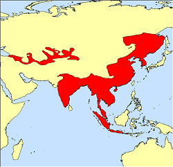
Step 1: Select the Unprojected Mode (see Toolbar above) to view the data in Latitude/Longitude co-ordinates. Step 2: Retrieve Tiger Population Data with the attribute Tiger Population. Aggregate on a yearly period. Tip: Change the layer properties to display the attribute as a colour palette. Double-click layer, select Colours Tab and check the palette option. Step 3: Animate using the animation icon. |
Volcano Images
|
Step 1: Select the Unprojected Mode (see Toolbar above) to view the data in Latitude/Longitude co-ordinates. Step 2: Retrieve Volcano Images with the attribute Shuttle Imaging Radar. Step 3: To view an image click on the Show File/Image/Movie icon and then click on a symbol on the map. |
| Browser Based Help. Published by chm2web software. |